Steps in SARIMA Based Time Series Forecasting For Electricity Demand Data
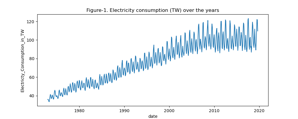
The data provided to us has two columns: date and electricity consumption in terra watts (Figure-1). The electricity consumption is provided to us in monthly intervals beginning in January 1973 and ending in December 2019. When plotted we observe that the data has an increasing trend in electricity usage from left to right with increasing time. We also observe that the increase is not in a linear fashion, indicating that there might be some seasonality or other cyclical patterns, which may be contributing to fluctuations around the general trend. One trend that comes to mind with electricity use and seasonality with monthly data is a trend lasting 12 monthly periods.
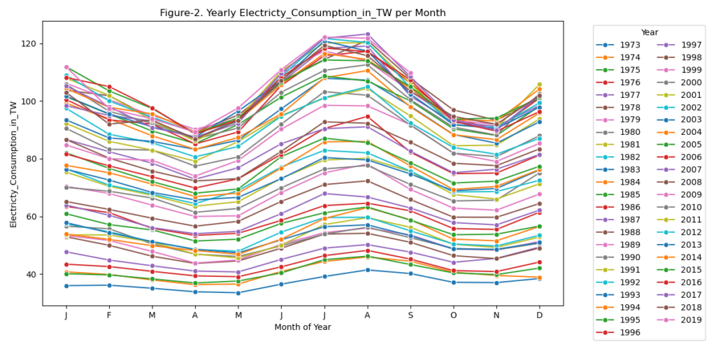
As soon as we plot each year’s monthly electricity usage (Figure-2), it becomes clear that there is a seasonality component to electricity usage that is conserved from the earliest time (1973, lowest blue line) to the most recent time (2019, salmon-colored line almost on top). In the next steps, we will determine whether– (i) this yearly increase in electricity usage is significant and quantifiable, (ii) then we will attempt to decompose the electricity consumption into trend, seasonality and residuals, followed by (iii) creation of model for forecasting, and we will conclude by discussing other factors and modeling techniques that might help better forecasting.
Dickey-Fuller Test: A statistical test used to determine whether a time series has a unit root, indicating that it is non-stationary. The non-stationarity can manifest as a series where the mean may drift over time, and variance may increase without bound. The presence of a unit root also suggests that past shocks may have a permanent influence on future values, leading to long-term dependencies.
Reference: Dickey, D. A., & Fuller, W. A. (1979). Distribution of the estimators for autoregressive time series with a unit root. Journal of the American Statistical Association, 74(366a), 427–431. Implementation: adfuller() is part of statsmodels.tsa.stattools
Null Hypothesis: A unit root is present in the time series, meaning the series is non-stationary. The alternative hypothesis is that the series is stationary.
Test Results: The null hypothesis is accepted and the series is not stationary. Meaning that the upward trend we see is true. But before we go into decomposition of trend and seasonality lets discuss the test statistics–
- Test Statistic: -1.8606, is greater than critical value at 1% and above (see below) therefore we cannot reject the null hypothesis that the time series is not stationary.
- p-value: 0.3408, this is a very high p-value indicating that the null hypothesis cannot be rejected. A value less than 0.05 would have indicated that the null hypothesis can be rejected.
- Lags Used: 12
- Number of Observations: 548
- Critical Values: 1% (-3.4423), 5% (-2.8669), 10%(-2.5696)
- AIC: 2329.7612, a lower value suggests a better fit and this can be used to compare results from different tests using distinct lag values.
Decomposition into trend and seasonality:
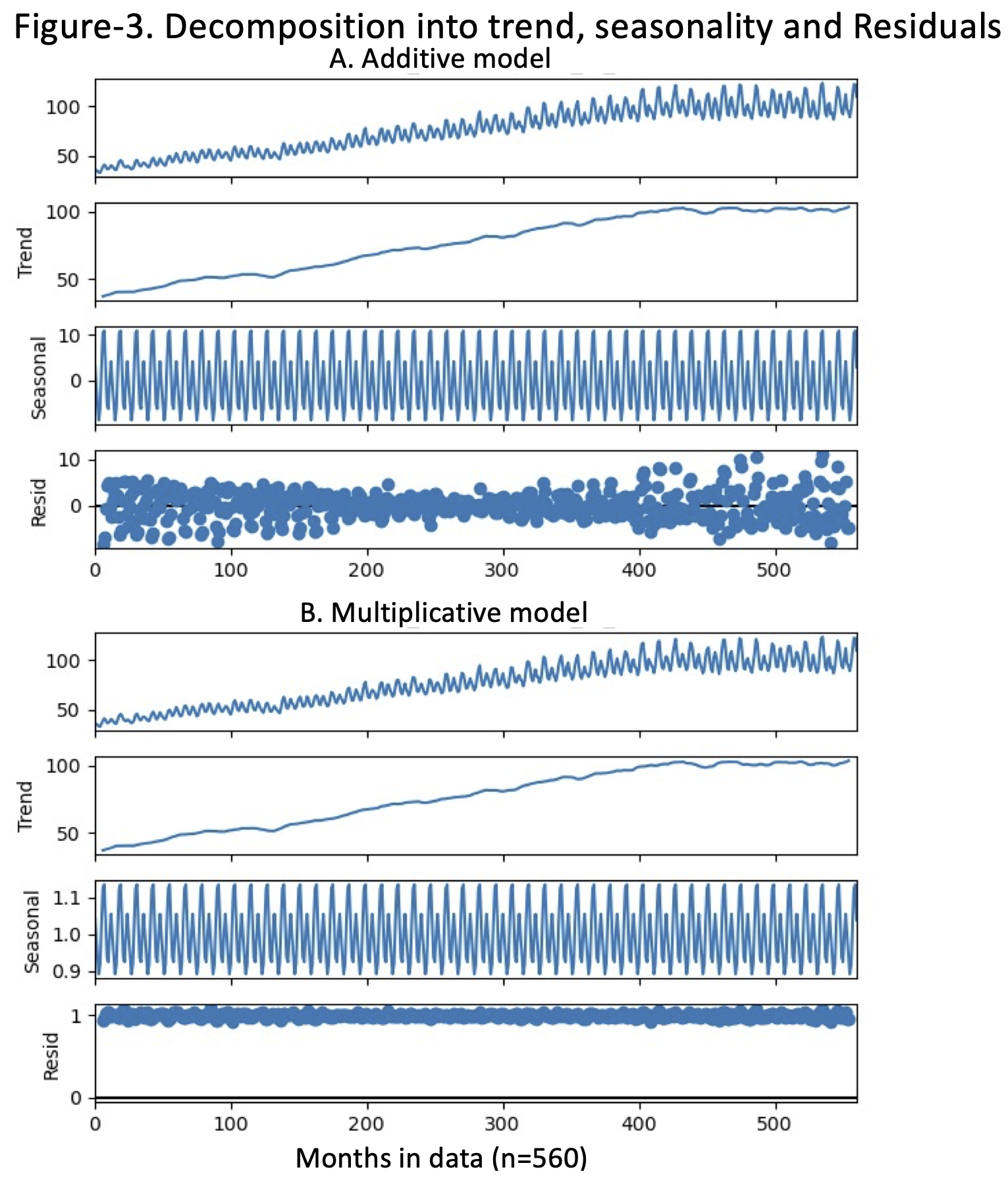
Is it additive or multiplicative?
- resource for whether it is additive or multiplicative.
- I believe it is multiplicative as residuals fluctuate around 1 in multiplicative suggesting that the multiplicative model captures the seasonal fluctuations well. In the multiplicative model, the residuals are expressed as a ratio, so a fluctuation around 1 implies that the seasonal component is proportional to the level of the time series.
- Usually, we would consider the seasonal part more, but in both analyses, the seasonal component is within the same range from beginning to end.
The Auto correlation function (ACF): Correlation of a time series with a lagged version of itself. It helps understand the order of Moving Average (MA) in ARIMA models.
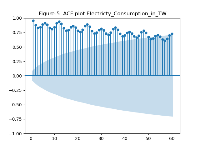
- lag is plotted on the x axis (x-axis = 1 is close to 1 on y-axis which means that there is almost 1 correlation of the time series with the series created by lagging by one. In other words, series from 0-59 months correlates closely with series from 1-60 months)
- the translucent area is area of no significance (any points falling in that area are of no significance, i.e, after a lag of 50 months the auto-correlation is pointless)
- Only the dots outside the translucent are significant.
- dots are the measures of correlation
- so I guess lag after 24 months it is becoming pointless to carry on the analysis
- and at 60 it is insignificant
- The ACF plot measures the influence of X point and all the other points between X and target. So if we are looking for effect of 10th interval, it is actually effect of 1-10 intervals.
- Look also at the seasonality in the data, we definitely need SARIMAX (below)
Partial Auto-Correlation Function (PACF) measures the correlation between a time series and its lagged values, while controlling for the influence of any correlations at shorter lags. In other words, it isolates and shows the direct relationship between the time series and each lagged value, excluding the effects of intermediate lags. PACF is useful for identifying the order of the Auto Regressive (AR) component in ARIMA models
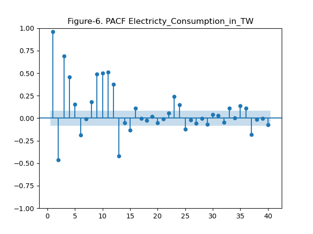
So here some months particularly 9-12 months before the ‘0’ month show significant correlation. Again, suggesting an annual seasonal component.
SARIMAX: Seasonal Auto Regressive Integrated Moving Average with eXogenous regressors Model
Well we dont have an X so we will use a SARIMA model without the X. But what could comprise an X? X could be – Weather features (temperature, humidity, precipitation), Calendar Effects (Day of the Week, Public Holidays, Seasonality), Energy Prices, Economic Indicators, Population Demographics, Technology and energy efficiency, Industrial and Commercial Activity. But today we will not go into these factors.
The SARIMAX equation is –
yt=μ+ϕ1yt−1+ϕ2yt−2+⋯+ϕpyt−p−θ1ϵt−1−θ2ϵt−2−⋯−θqϵt−q+Φ1yt−s+Φ2yt−2s+⋯+ΦPyt−Ps−Θ1ϵt−s−Θ2ϵt−2s−⋯−ΘQϵt−Qs+β1x1t+β2x2t+⋯+βkxkt+ϵt
Where:
- yt is the value of the time series at time t.
- μ is the intercept.
- ϕi are the parameters of the non-seasonal autoregressive (AR) terms.
- θi are the parameters of the non-seasonal moving average (MA) terms.
- Φi are the parameters of the seasonal autoregressive (SAR) terms.
- Θi are the parameters of the seasonal moving average (SMA) terms.
- s is the length of the seasonal cycle.
- βi are the coefficients of the exogenous variables xit.
- ϵt is the error term (white noise).
Simplified Notation
The SARIMAX model can also be summarized using the notation (p,d,q)×(P,D,Q)s with exogenous regressors, where:
- p is the order of the non-seasonal AR terms. (number of non seasonal lag observations to use)
- d is the order of non-seasonal differencing. (number of times raw observations are differenced)
- q is the order of the non-seasonal MA terms. (size of the moving average window)
- P is the order of the seasonal AR terms. (number of seasonal auto regressive terms to use)
- D is the order of seasonal differencing. (number of seasonal differences to use)
- Q is the order of the seasonal MA terms. (number of seasonal moving average terms)
- s is the length of the seasonal cycle. (12 for monthly data with an annual seasonal cycle)
This representation helps in understanding and communicating the structure of the model clearly.
SARIMA: employed with auto_arima to determine best set of hypervariables
I used the auto_arima function from pmdarima.arima to iterate through multiple hypervariables and find the most suited hyper-variables. Here, I used
- m=12 ## for 12 month seasonality
- max_order = None ## to use all combinations of p and q
- max_p = 7 ## to use a maximum of 7 non seasonal lags for AR (ref. ACF)
- max_q = 7 ## to use a maximum of 7 non seasonal lags for MA (ref. PACF)
- max_d = 2 ## max d to use, 2 avoids overfitting in most cases
- max_P = 4 ## to use up to 4 year old data for prediction as after 50 months the significance dropped
- max_Q = 4 ## same reason as above
- max_D = 2 ## same as max_d
- alpha=0.05 ## specifies significance level for statistical tests
- trend = “ct” ## to include both constant and linear trend
- information_criterion = ‘oob’, ## (out-of-bag) criterion evaluates model performance on a held-out sample of data
- out_of_sample = int(len(elec_df)*0.2)) ## means that 20% of the data will be used for validation
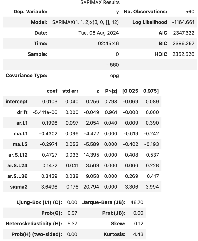
The model with best outcome –
Model: SARIMAX(1, 1, 2)x(3, 0, [], 12)
- SARIMAX(1, 1, 2): Non-seasonal part
- AR(1): 1 autoregressive term.
- MA(2): 2 moving average terms.
- d = 1: 1 non-seasonal differencing.
- x(3, 0, [], 12): Seasonal part
- SAR(3): 3 seasonal autoregressive terms.
- SMA = []: No seasonal moving average terms.
- D = 0: No seasonal differencing.
- s = 12: Seasonal period (e.g., 12 months for monthly data).
SARIMAX Model Equation
The SARIMAX model combines autoregressive (AR), moving average (MA), and seasonal autoregressive (SAR) components. The combined equation is:
— Need to work on Latex and/or Math jax for WordPress —
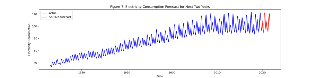
And finally, our prediction-